Deep Reinforcement Learning on Space Invaders Using Keras
Full code for training Double Deep \(Q\) Network and Duel \(Q\) Network
Over the winter break I thought it would be fun to experiment with deep reinforcement learning. Using the ideas of reinforcement learning computers have been able to do amazing things such master the game of Go, play 3D racing games competitively, and undergo complex manipulations of the environment around them that completely defy explicit programming!
A little under 3 years ago, Deepmind released a Deep \(Q\) Learning reinforcement learning based learning algorithm that was able to master several games from Atari 2600 sheerly based of the pixels in the screen of the game. In this blog, we will test out the Deep \(Q\) network on the Atari game Space Invaders, using OpenAI Gym, incorporating a couple newer architecture changes proposed in more recent papers, Dueling Deep \(Q\) networks (DQN) and Double Deep \(Q\) networks (DDQN).
Background
Suppose that you are located somewhere in an unknown grid. At any timestep you may only move up, right, down or left. Each resulting action will give some amount of reward. Your oal is to the find the optimal set of moves so that you will have the maximum amount of award after \(T\) timesteps. Doesn’t sound that bad? Sure, but what if you were only given a limited number trials to explore moves? Furthermore, what if the rewards were very sparse? Perhaps you will only start getting rewards after the 20th move despite the fact that it was your second move that was crucial for you get a reward.
The above situation is exactly an example of a problem in reinforcement learning. In reinforcement learning, we are given a set of possible states and actions. We assume that a state will have the same set of actions regardless of our moves previously to get to the state. We then wish to find the optimum behavior such that some reward is maximized. We define \(V_s\) given a state \(s\) to be equal to the amount of total award we can get from state \(s\) assuming optimal movement. That is
\[\begin{align*} V_s = \max \sum_{t=0}^T R_t \end{align*}\]where \(R_0\) denotes the amount of award received in the first timestep and so forth.
Note however that the above equation does not generalize when we could potentially play forever. If we allow \(T\) to approach infinity, then the sum will always approach infinity. However, we wish to differentiate between all strategies that are infinitely long. To deal with this problem we introduce a discount factor \(\gamma\) and multiply the reward we get at each future timestep by multiplicative factors of \(\gamma\). As we view results much
\[\begin{align*} V_s = \max \sum_{t=0}^{\infty} \gamma^tR_t \end{align*}\]further in the future, their value will then be exponentially decreased by \(\gamma\), effectively minimizing rewards in the far future. This can also be justified by decreased confidence in the future.
\(Q\) Value
An alternative method to assigning values to states is to assign values to state, action pairs instead of just states. Specifically, we define \(Q(s,a)\) to be equal to the total amount of discounted reward that we can get if we are initially in states \(s\) and do action \(a\). We refer to \(Q(s,a)\) for an action \(a\) as the \(Q\) value of the action. Assume doing some action a leads to subsequent state \(s'\), then note that we have the following:
\[\begin{align*} Q(s,a) = r(s,a)+\gamma \max_a Q(s', a) \end{align*}\]where \(r(s,a)\) is the reward received from being in state \(s\) and doing action \(a\). The above equation is true since when we reach state \(s'\), the action with the maximum \(Q\) value will be the optimal to take to maximize reward.
In normal reinforcement learning under \(Q\) learning, we wish to calculate the value of \(Q(s, a)\) for all values of s and a. Deep reinforcement learning is pretty similar, except that our state consists of the pixel values of the screen. This allows our reinforcement learning algorithm to easy generalize to any game that can be displayed on a screen. Unfortunately, if we were to try to explicitly construct a table for all possible values of s and a, it would absolutely gigantic. If we take our state as the last 3 frames in a game with screen size 100 by 100, we would have over \(10^{12}\) possible states!
Fortunately though, if we are using pixels as the possible states that we are in, there is likely a lot of repetition in our states where two very similar states are likely to have the same \(Q\) value. Neural networks are very good at learning functions on these repetitive states. In repetitive image processing, convolutional neural networks(CNN) are the method of choice. Therefore, we construct a CNN whose input is the state of the last couple frames of the game and whose output layer is the estimated \(Q\) values for the list of possible actions. A tutorial on CNN can be found here
Deep \(Q\) Learning
As mentioned above in deep \(Q\) learning, we construct a CNN to process input states and output \(Q\) values for possible actions. For the particular game of space invaders , we construct a network of the following architecture.
| Name | Input Shape | Filter Size | Filter Number | Stride | Output Shape |
|---|---|---|---|---|---|
| conv1 | 3x84x84 | 8x8 | 32 | 4 | 32x20x20 |
| conv2 | 32x20x20 | 4x4 | 64 | 2 | 64x9x9 |
| conv3 | 64x9x9 | 3x3 | 64 | 1 | 64x7x7 |
| flatten | 64x7x7 | - | - | - | 512 |
| fc1 | 512 | - | - | - | 6 |
where we set the final output layer to be equal to 6 since this is the number of actions our agent is allowed to move.
We can implement the CNN in Keras using the following code:
    def construct_q_network(self):
        self.model = Sequential()
        self.model.add(Convolution2D(32, 8, 8, subsample=(4, 4), input_shape=(84, 84, NUM_FRAMES)))
        self.model.add(Activation('relu'))
        self.model.add(Convolution2D(64, 4, 4, subsample=(2, 2)))
        self.model.add(Activation('relu'))
        self.model.add(Convolution2D(64, 3, 3))
        self.model.add(Activation('relu'))
        self.model.add(Flatten())
        self.model.add(Dense(512))
        self.model.add(Activation('relu'))
        self.model.add(Dense(NUM_ACTIONS))
One interesting thing to note is that we are missing a max pooling layer that is usually found in CNNs for vision detection. This is because max pooling is primarily used to implement translational invariance – which we don’t really care about in a convolution neural network.
Another thing to note is that our CNN takes as input a image of size 84x84. This is different then the default resolution of the Atari gamescreen of 192 by 160. This is to make training computationally easier. Furthermore, we convert each input image of 3 RGB channels to 1 black white channel since color doesn’t really effect gameplay. Finally, for each input image into our CNN, we stack the last three frames that have occured – this way we can sense if a bullet is falling down.
The code for converting the last three frames to one single channel image is below:
    def convert_process_buffer(self):
        """Converts the list of NUM_FRAMES images in the process buffer
        into one training sample"""
        black_buffer = map(lambda x: cv2.resize(cv2.cvtColor(x, cv2.COLOR_RGB2GRAY), (84, 90)), self.process_buffer)
        black_buffer = map(lambda x: x[1:85, :, np.newaxis], black_buffer)
        return np.concatenate(black_buffer, axis=2)
In the above code, self.process_buffer contains the last three full sized 192x160x3 pictures.
Replay Buffer
A problem when we are training our network is the fact that if we only train on frames of data as they come in, we would be overfitting on the last few frames of the data. As a result, we keep a buffer of all the last 20000 experiences we have experienced so far and randomly sample a batch of 64 images to learn on at each step of the game. This way, we won’t overfit on the most recent frames. This is called experience replay.
Experience replay is also found biologically! Studies in rats have shown that replay of events is vital for rats to learn tasks. Specifically, they found that selective emphasis of replay of surprising events in the past. One possible incorporation of this fact into our network is to replay past events, but with increased emphasis on events with high temporal difference(events that are very different than what we expect) as done in the paper here We use the following data structure for our replay buffer.
class ReplayBuffer:
    """Constructs a buffer object that stores the past moves
    and samples a set of subsamples"""

    def __init__(self, buffer_size):
        self.buffer_size = buffer_size
        self.count = 0
        self.buffer = deque()

    def add(self, s, a, r, d, s2):
        """Add an experience to the buffer"""
        # S represents current state, a is action,
        # r is reward, d is whether it is the end,
        # and s2 is next state
        experience = (s, a, r, d, s2)
        if self.count < self.buffer_size:
            self.buffer.append(experience)
            self.count += 1
        else:
            self.buffer.popleft()
            self.buffer.append(experience)

    def size(self):
        return self.count

    def sample(self, batch_size):
        """Samples a total of elements equal to batch_size from buffer
        if buffer contains enough elements. Otherwise return all elements"""

        batch = []

        if self.count < batch_size:
            batch = random.sample(self.buffer, self.count)
        else:
            batch = random.sample(self.buffer, batch_size)

        # Maps each experience in batch in batches of states, actions, rewards
        # and new states
        s_batch, a_batch, r_batch, d_batch, s2_batch = map(np.array, zip(*batch))

        return s_batch, a_batch, r_batch, d_batch, s2_batch
Exploration
How do we play the game while we are training our network? Do we continuously choose what we believe is the best action? But if we do this , how will we be able to discover a new move? This general problem is known and exploration vs exploitation tradeoff. We remedy this problem, we use an \(\epsilon\) exploration policy to play the game. This means that with probability \(\epsilon\) you do a random action. Otherwise, we select the action with the highest \(Q\) value(what we believe is the best action) from our current state. In addition, since at the beginning of training, our belief in \(Q\) values is completely baseless, we slowly linearly decrease our \(\epsilon\) from \(1\) to \(0.1\). We can do this in code as follows.
    def predict_movement(self, data, epsilon):
        """Predict movement of game controler where is epsilon
        probability randomly move."""
        q_actions = self.model.predict(data.reshape(1, 84, 84, NUM_FRAMES), batch_size = 1)
        opt_policy = np.argmax(q_actions)
        rand_val = np.random.random()
        if rand_val < epsilon:
            opt_policy = np.random.randint(0, NUM_ACTIONS)
        return opt_policy, q_actions[0, opt_policy]
Loss Function and Target Networks
As mentioned above, we wish that each of the outputs of our CNN be equal to the \(Q\) value of a respective action. We know from this fact that outputs should satisfy that
\[\begin{align*} Q(s,a) = r+\gamma \max_a Q(s', a) \end{align*}\]Therefore, for every \((s, a, r, s')\) action tuple in our replay buffer we minimize the discrepancy between the \(Q\) value predicted directly from the neural network and the \(Q\) value constructed from the subsequent reward and maximum \(Q\) value of the resultant state, if the state is non-terminal. If the state is terminal, then the expect \(Q\) value should just be the reward. I used MSE(mean square error) as a loss function. This can be implemented in Keras below
    def train(self, s_batch, a_batch, r_batch, d_batch, s2_batch, observation_num):
        """Trains network to fit given parameters"""
        batch_size = s_batch.shape[0]
        targets = np.zeros((batch_size, NUM_ACTIONS))

        for i in xrange(batch_size):
            targets[i] = self.model.predict(s_batch[i].reshape(1, 84, 84, NUM_FRAMES), batch_size = 1)
            fut_action = self.target_model.predict(s2_batch[i].reshape(1, 84, 84, NUM_FRAMES), batch_size = 1)
            targets[i, a_batch[i]] = r_batch[i]
            if d_batch[i] == False:
                targets[i, a_batch[i]] += DECAY_RATE * np.max(fut_action)

        loss = self.model.train_on_batch(s_batch, targets)
Note that in the above code, we actually use a second “target” network to predict the Q values of the transitioned state \(s'\). The second “target” network is set to the weights of the original network every so many frames but is otherwise unchanged. This allows the deep \(Q\) network to converge more quickly, since otherwise we could enter a self feedback loop where we continuously estimate higher and higher \(Q\) values. The code for setting the weights of the target network is below
    def target_train(self):
        model_weights = self.model.get_weights()
        self.target_model.set_weights(model_weights)
Results for Double Deep \(Q\) Network
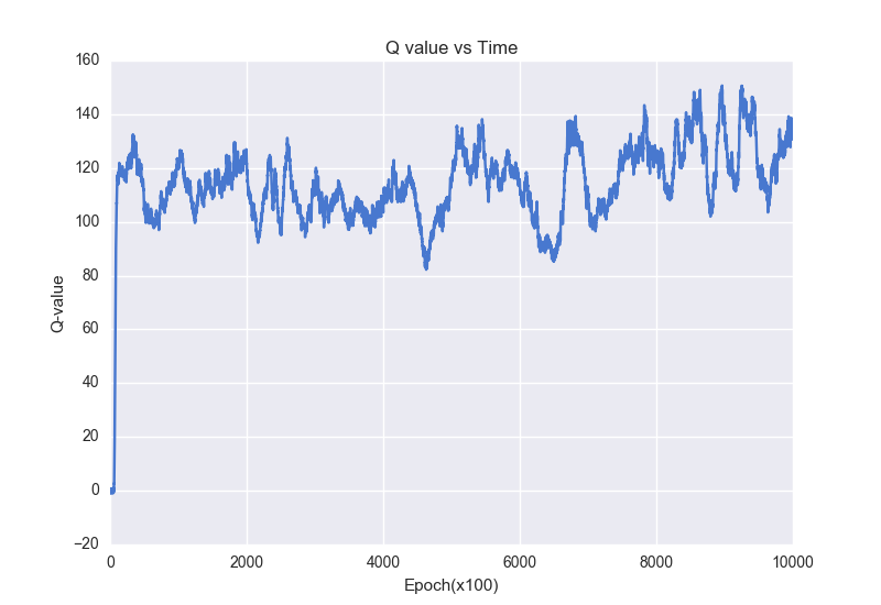
Combining all the code above we construct a Double Deep \(Q\) Networks(the target network is our “second” network) , after training for about 1,000,000 frames, we get an average score of around 260 on the game of space invaders(full code can be found here). Below is a video of the Double Deep \(Q\) Network playing.
We can visualize \(Q\) values of different actions as we train the DDQN, which is shown in the plot below. Loosely, these Q values can represent how our network is learning how to play this game.
Dueling \(Q\) Network
One problem with our above implementation of a Deep \(Q\) Network is that we are currently directly estimating the value of being at a state and executing a specific action. However, much of the time, the value of doing any action doesn’t really influence the value of being at a specific state. In a dueling \(Q\) network architecture, we seek to separate
\[\begin{align} Q(s,a) = A(s,a) + V(s) \end{align}\]where under this definition, \(A(s,a)\) will represents the advantage of making a certain action and \(V(s)\) will represents the current value of being at a certain state.
How do we do this? We construct two separate two streams in our CNN - one to estimate the value of a state and another to estimate the advantage of each of the actions. Note that both streams share the same weights for the convolutional layers. We then combine these layers to predict the \(Q\) values of each action. Unfortunately, directly summing these separate streams gives us no guarantees that the first stream will actually predict the value of a state. Instead we combine them with criterion
\[\begin{align} Q(s,a) = V(s) + A(s,a) - \frac{1}{\|a\|}\sum_{a'}A(s,a') \end{align}\]Under the above criterion, on average, the advantage stream will be on average equal to 0, leading the value stream to approximately predict the value of the state.
We can implement this in Keras using the following code
    def construct_q_network(self):
        # Uses the network architecture found in DeepMind paper
        self.model = Sequential()
        input_layer = Input(shape = (84, 84, NUM_FRAMES))
        conv1 = Convolution2D(32, 8, 8, subsample=(4, 4), activation='relu')(input_layer)
        conv2 = Convolution2D(64, 4, 4, subsample=(2, 2), activation='relu')(conv1)
        conv3 = Convolution2D(64, 3, 3, activation = 'relu')(conv2)
        flatten = Flatten()(conv3)
        fc1 = Dense(512)(flatten)
        advantage = Dense(NUM_ACTIONS)(fc1)
        fc2 = Dense(512)(flatten)
        value = Dense(1)(fc2)
        policy = merge([advantage, value], mode = lambda x: x[0]-K.mean(x[0])+x[1], output_shape = (NUM_ACTIONS,))

        self.model = Model(input=[input_layer], output=[policy])
Results for Duel \(Q\) Network
Under the Duel \(Q\) Network, after about 600,000 frames of training, I got an average score of 297, better than the DDQN. Interestingly, the movement is also very different then the Deep \(Q\) Network(I tried several different initializations of both networks and seemed to always result in these distinctive behaviors of play)!

Conclusion
In the above blog post, we explored how we can use Deep \(Q\) Networks to achieve decent performance on the Space Invaders game. Given additional training time, the performance on the tasks will probably increase.
As a final word, there are many possible improvements we can make on the architecture described. One interesting possibility, inspired partly from cognitive science, is prioritized replay, where we seek to preferentially replay events that are very ‘different’(our estimated \(Q\) values significantly different than actual \(Q\) values) from what we expect. Recently, Google DeepMind released Asynchronous Advantage Actor Critic (A3C) method which generally performs better than variants of DQN on almost all games in the Atari suite, including Space Invaders.
Acknowledgments
This blog post would not be possible without so many amazing resources online! Code from here and here were used as references for the code presented above.
There were a lot of parts of code in the above implementation and if there were any errors please let me know!