A3C and Policy Bots on Generals.io in Pytorch
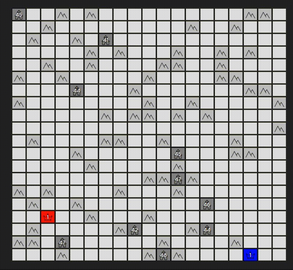
Full code for A3C training and Generals.io Processing and corresponding replay. Blue player is policy bot.
Generals.io is a game where each player is spawned on an unknown location in the map and is tasked with expanding their land and capturing cities before eventually taking out enemy generals. What makes the game of generals environment interesting is that it is a imcomplete information game where each player is unaware of the actions of other players except when boundaries collide. Over the past 8 or so months I’ve had a lot of fun playing the game. Inspired by the AlphaGo paper, I decided to construct a series of networks towards playing the game of generals.io.
Background
Value Function Estimation
Loosely, there are three different approaches towards deep reinforcement learning. The first, value function estimation, aims to estimate the approximate value of various states based off the expected rewards it will get in the future. Since typically our algorithms are model-free, with just an value function estimate of a state, we are unfortunately unable to determine what action to take to actually reach a better state. As a result, a modified version of value function estimation is used where we estimate the Q value or reward of a state and action pair. At test time, we then choose the action that has the highest reward with the current state. Networks of this type include, deep Q networks, dueling Q network and many such variants. Details can be found at the previous blog post
Policy Estimation
A second approach towards deep reinforcement learning regards policy estimation. A policy \(\pi\) maps a state \(s\) to a set of actions \(a\). Policy estimation involves directly estimating a policy for every state. In constract to value function estimation, where we estimate a policy based off values of state such as Q values, we derictly estimate policy based off discounted rewards of a particular action. Generally, we estimate a policy gradient for a particular action based off the discounted reward of the action, policy estimation can actually be used without computing any gradients at all by just choosing the best policy out a group of competing policies. Traditionally, policy gradient algorithms have been used for discrete action spaces with stochastic policies through the Reinforce algorithm by randomly sampling each action, the deterministic policy gradient theorem allow policy gradients to be calculated even in deterministic policies, allowing estimation of policies on continuous actions in environments such as TORCS(simulated driving).
Actor Critic Network
A third approach towards deep reinforcement learning regards the actor critic model,used in this network, where we combine both policy estimation and value estimation. This combination allows actor critic models to be applicable in both discrete and continuous action from policy estimation while value estimation allows us to reduce variance in training. This combination allows us to get good results on many RL environments, especially when multiple networks are trained. We describe actor critic networks in more detail below.
The actor critic network can roughly be described in the diagram below
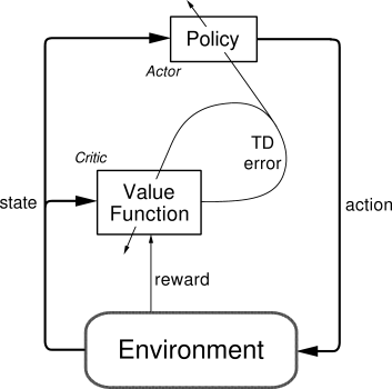
We approximate both policy and value functions with neural networks which we denote with \(\pi_{\theta}(s, a)\) and \(V_w(s)\). We run value and policy networks for multiple iterations. We then choose the loss of the value network to be equal to
\[\begin{align*} L_v = \sum (R - V(s))^2 \end{align*}\]where we define the \(R\) equal to the discounted reward of each individual reward plus a value network estimate of the last state
\[\begin{align*} R = \sum \gamma^i r_i + V(s_t) \end{align*}\]where \(s_t\) is the terminal state and the \(\gamma\) is the discount factor for subsequent states. We then train the policy network using generalized advantage of each action.
We define advantage as \(A(s) = R - V(s)\). To reduce the variance of advantage estimates, we use generalized advantage, which is an exponential mean of subsequent advantages defined as
\[\begin{align*} GAE(s) = (1-\tau)\sum A(s) \tau^t * \gamma^t \end{align*}\]where the parameter \(\tau\) specifies the contribution of future advantage estimates
We then define the policy loss as
\[\begin{align*} L_p = \sum (-\log{a_i}*GAE(a_i) + c * H(a)) \end{align*}\]where \(a_i\) specifies the probability of taking action \(i\) while \(H(a)\) specifies the entropy of an action choice. An entropy penalty term is added to the loss function to ensure exploration of all actions.
In practice and in our networks, models share the same early layers with diverging final layers. Following the A3C paper published by DeepMind, we train on network asynchronously on CPU using a total 16 CPU cores.
Generals Game State Simulation and Preprocessing
To allow generate datasets and to create a generals environment for bots to play against each other we construct to utility classes to simulate a replay file and to generate generals environment with another bot playing at here and here respectively.
To make the original board state more informative to a bot, we expand the original board state into multiple different seperate input channels. As I didn’t try many different feature expansions, there might be various other feature expansions that may significantly improve performance.
We describe the features below:
| Feature Number | Description |
|---|---|
| 0 | army values on friendly tiles |
| 1 | army values on enemy tiles |
| 2 | indicators for obstacles(mountain/cities) |
| 3 | army values on neutral cities |
| 4 | indicator for mountains |
| 5 | indicator for generals |
| 6 | indicator for not visible locations |
| 7 | army values for self owned cities |
| 8 | army values for enemy owned cities |
| 9 | turn number % 50 |
| 10 | ratio of enemy troops to own troops |
Another thing to note is that order of magnitude of features are very different, which may lead a network to prioritize certain features over other.
Policy Network Architecture and Training
The first network we train is the policy network based on past general games played between players found here. Using the code found here, we construct a dataset containing approximately 11,000 games between 1v1 matches between players with stars over 90.
We define a architecture to the policy network below:
class CNNLSTMPolicy(nn.Module):

    def __init__(self, on_gpu = False):
        super(CNNLSTMPolicy, self).__init__()
        self.lstm_layer = 3
        self.hidden_dim = 100
        self.on_gpu = on_gpu

        self.conv1 = nn.Conv2d(11, self.hidden_dim, 5, padding=2)

        self.conv2 = nn.Conv2d(self.hidden_dim, self.hidden_dim, 5, padding=2)
        self.conv3 = nn.Conv2d(self.hidden_dim, self.hidden_dim, 5, padding=2)

        self.pre_lstm_bn = nn.BatchNorm2d(self.hidden_dim)

        self.lstm = nn.LSTM(self.hidden_dim, self.hidden_dim, self.lstm_layer)

        self.lstm_batch_norm = nn.BatchNorm2d(self.hidden_dim)

        self.conv4 = nn.Conv2d(self.hidden_dim, self.hidden_dim, 5, padding=2)
        self.conv5 = nn.Conv2d(self.hidden_dim, self.hidden_dim, 5, padding=2)

        self.begin_conv = nn.Conv2d(self.hidden_dim, 1, 1)
        self.end_conv = nn.Conv2d(self.hidden_dim, 2, 1)

    def init_hidden(self, height, width):
        self.height = height
        self.width = width
        self.batch = height * width

        self.cell_state = Variable(torch.zeros(self.lstm_layer, self.batch, self.hidden_dim))
        self.hidden_state = Variable(torch.zeros(self.lstm_layer, self.batch, self.hidden_dim))

        if self.on_gpu:
            self.cell_state = self.cell_state.cuda()
            self.hidden_state = self.hidden_state.cuda()

    def forward(self, input):
        # TODO perhaps add batch normalization or layer normalization

        x = F.elu(self.conv1(input))
        x = F.elu(self.conv2(x))
        x = F.elu(self.conv3(x))

        # Next flatten the output to be batched into LSTM layers
        # The shape of x is batch_size, channels, height, width
        x = self.pre_lstm_bn(x)

        x = torch.transpose(x, 1, 3)
        x = torch.transpose(x, 1, 2)
        x = x.contiguous()

        x = x.view(x.size(0), self.batch, self.hidden_dim)
        x, hidden = self.lstm(x, (self.hidden_state, self.cell_state))
        self.hidden_state, self.cell_state = hidden

        x = torch.transpose(x, 2, 1)
        x = x.contiguous()
        x = x.view(x.size(0), self.hidden_dim, self.height, self.width)

        x = self.lstm_batch_norm(x)

        x = F.elu(self.conv4(x))
        x = F.elu(self.conv5(x))

        o_begin = self.begin_conv(x)
        o_end = self.end_conv(x)

        o_begin = o_begin.view(o_begin.size(0), -1)
        o_end = o_end.view(o_end.size(0), -1)

        o_begin = F.log_softmax(o_begin)
        o_end = F.log_softmax(o_end)

        return o_begin, o_end
Architecture for Policy Bot
A turn of a generals.io game requires a bot to choose a tile from which we select a movement direction for an army. Roughly our model can be described as 3 5x5 padded convolutions followed by a 3 layer LSTM on each individual tile followed by 2 5x5 padded convolutions leading to two indepedent map sized outputs representing the start and end tiles for moving an army.
Architecture Design Choices
Since the size of game board is variable, we choose to use a full convolutional network that predicts both the most likely start and end tiles for an army movement. We choose to use a fully convolutional architecture as opposed to variable size max-pooling to account for different sizes so that we can add an intermediate LSTM representation on each independent tile of the board to store possible states of tiles.
We choose to output start and end army movement tiles as opposed to an army tile and movement direction to reduce the number of possible actions. In addition, in this way way, the bot is able to focus on the first output, the potential army locations to move and in the second output, places to move to seperately. Dependent on the situation, the first output might be important for rapid expansion movement while the second output could be useful for choosing targets for attacking or reinforcement.
We choose to add 3 layers of LSTM encoding on each individual tile of the generals.io map to allow the network to have the ability to remember events that occured in specific locations of a tile since vision to locations on map can dissapear if nearby armies are wiped away. This can allow the policy network to undergo continous attacks on an enemy general location or two actively defend its own general location.
We add batch normalization to our network to prevent covariate shift(which appeared to reduce training error significantly). I also tried adding residual connections between layers, although it appeared it increase final training loss.
After initializing weights for networks, the network was trained by feeding the network one batch of board states from one generals game after another through a total of 2 epochs using the Adam optimizer.
Performance Analysis of Policy Bot
A link to the bot playing a game of generals.io is shown here. To generate a move prediction given a board state we feed the expanded board state to the bot and ask it to predict the most likely tile to start a move from and to end a move from. We then find the valid move pair with the highest likelihood of moving from start to end from.
The bot appears to be able to effectively expand and take surrounding cities. The bot was trained on greater than 90 star 1v1 generals games, which may explain city taking by the bot. Unfortunately, it does not appear that independent LSTMs on each seperate tile on the grid enabled the bot to make solid objective based choices, and the bot unable to make targeted attacks against generals. This may have been due partly to the fact the bot was only trained to predict movements one step in the future.
Reinforcement Learning Training with A3C
Looking into the bot trained through supervised movements of players playing the bot, it appeared as if the bot had obtained a general idea of the environment around it, being able to effectively expand and take surrounding neutral cities. However, it does not appear as if the bot actually understand the objective of the game and was not able to follow more advanced human strategies such as concerted charges or continuous defense of ones general upon discovery by enemy generals.
My thoughts were that if we were to reinforcement train the bot by playing it against its self, it would eventually learn long distance patterns through which it could defeat its opponent. As a result, I created an OpenAI Gym like environment for generals, with a bundled policy network movement predictor. The goal of the new network, an actor critic network, was to maximize its respecitive reward given the enviroment. I chose to give the bot rewards every time it captured either a tile, a city or an enemy general.
To choose a network learn under the reinforcement learning general environment, I chose to use an advantage actor critic network. The code for the actor critic network is given below:
class ActorCritic(nn.Module):

    def __init__(self, on_gpu = False):
        # Current architecture for policy is 3 5x5 convolutions
        # followed by 2 LSTM layers followed by 2 5x5 convolutions
        # and a final 1x1 convolution
        # This architecture if fully convolutional with no max pooling
        super(ActorCritic, self).__init__()
        self.lstm_layer = 3
        self.hidden_dim = 150
        self.on_gpu = on_gpu

        self.conv1 = nn.Conv2d(11, self.hidden_dim, 5, padding=2)

        self.conv2 = nn.Conv2d(self.hidden_dim, self.hidden_dim, 5, padding=2)
        self.conv3 = nn.Conv2d(self.hidden_dim, self.hidden_dim, 5, padding=2)

        self.pre_lstm_bn = nn.BatchNorm2d(self.hidden_dim)

        self.lstm = nn.LSTM(self.hidden_dim, self.hidden_dim, self.lstm_layer)

        self.lstm_batch_norm = nn.BatchNorm2d(self.hidden_dim)

        self.conv4 = nn.Conv2d(self.hidden_dim, self.hidden_dim, 5, padding=2)
        self.conv5 = nn.Conv2d(self.hidden_dim, self.hidden_dim, 5, padding=2)

        self.move_conv = nn.Conv2d(self.hidden_dim, 8, 1)
        self.value_conv = nn.Conv2d(self.hidden_dim, self.hidden_dim, 1)
        self.value_linear = nn.Linear(self.hidden_dim, 1)

    def init_hidden(self, height, width):
        self.height = height
        self.width = width
        self.batch = height * width

        self.cell_state = Variable(torch.zeros(self.lstm_layer, self.batch, self.hidden_dim))
        self.hidden_state = Variable(torch.zeros(self.lstm_layer, self.batch, self.hidden_dim))

        if self.on_gpu:
            self.cell_state = self.cell_state.cuda()
            self.hidden_state = self.hidden_state.cuda()

    def reset_hidden(self):
        # Zero gradients on hidden states
        self.cell_state = Variable(self.cell_state.data)
        self.hidden_state = Variable(self.hidden_state.data)

    def forward(self, input):
        x = F.elu(self.conv1(input))
        x = F.elu(self.conv2(x))
        x = F.elu(self.conv3(x))

        # Next flatten the output to be batched into LSTM layers
        # The shape of x is batch_size, channels, height, width
        x = self.pre_lstm_bn(x)

        x = torch.transpose(x, 1, 3)
        x = torch.transpose(x, 1, 2)
        x = x.contiguous()

        x = x.view(x.size(0), self.batch, self.hidden_dim)
        x, hidden = self.lstm(x, (self.hidden_state, self.cell_state))
        self.hidden_state, self.cell_state = hidden

        x = torch.transpose(x, 2, 1)
        x = x.contiguous()
        x = x.view(x.size(0), self.hidden_dim, self.height, self.width)

        x = self.lstm_batch_norm(x)

        x = F.elu(self.conv4(x))
        x = F.elu(self.conv5(x))

        logit = self.move_conv(x)
        logit = logit.view(logit.size(0), -1)

        x = self.value_conv(x)
        x = x.view(x.size(0), self.hidden_dim, self.batch)
        x = F.max_pool1d(x, self.batch)
        x = x.squeeze()
        val = self.value_linear(x)

        return val, logit
In training, we run multiple different reinforcement learning generals environment at a time, to allow an agent to simultaneously updated gradients to parameters while experiencing several different experiences.
To train each network, we step through the environment using the code below:
    while True:
        # Sync with the shared model
        model.load_state_dict(shared_model.state_dict())

        values = []
        log_probs = []
        rewards = []
        entropies = []
        off_targets = []

        for step in range(args.num_steps):
            episode_length += 1
            value, logit = model(Variable(state.unsqueeze(0)))
            prob = F.softmax(logit)
            old_prob = prob

            # Set the probability of all items that not owned by user to
            # 0
            army_map = state[0, ...]
            label_map = (army_map > 0)
            label_map = label_map.view(1, env.map_height, env.map_width)
            label_map = label_map.expand(8, env.map_height, env.map_width)
            label_map = label_map.contiguous()
            label_map = label_map.view(-1)
            # prob[~label_map] = 0
            prob = old_prob * Variable(label_map.float())
            # Penalize model for predicting off target tiles
            off_prob = old_prob * Variable((~label_map).float())
            off_targets.append(off_prob.sum(1))

            log_prob = F.log_softmax(logit)
            entropy = -(log_prob * prob).sum(1)
            entropies.append(entropy)

            action = prob.multinomial().data
            log_prob = log_prob.gather(1, Variable(action))

            state, reward, done, _ = env.step(action.numpy().flat[0])
            done = done or episode_length >= args.max_episode_length

            if done:
                episode_length = 0
                state = env.reset()
                model.init_hidden(env.map_height, env.map_width)

            state = torch.Tensor(state)
            values.append(value)
            log_probs.append(log_prob)
            rewards.append(reward)

            if done:
                break

        R = torch.zeros(1, 1)
        if not done:
            value, _ = model(Variable(state.unsqueeze(0)))
            R = value.data

        values.append(Variable(R))
        policy_loss = 0
        value_loss = 0
        R = Variable(R)
        gae = torch.zeros(1, 1)
        for i in reversed(range(len(rewards))):
            R = args.gamma * R + rewards[i]
            advantage = R - values[i]
            value_loss = value_loss + 0.5 * advantage.pow(2)

            # Generalized Advantage Estimataion
            delta_t = rewards[i] + args.gamma * \
                values[i + 1].data - values[i].data
            gae = gae * args.gamma * args.tau + delta_t

            policy_loss = policy_loss - \
                log_probs[i] * Variable(gae) - args.entropy_coef * entropies[i] + \
                args.off_tile_coef * off_targets[i]

        optimizer.zero_grad()
        loss = policy_loss + args.value_loss_coef * value_loss

        (loss).backward()
        torch.nn.utils.clip_grad_norm(model.parameters(), args.max_grad_norm)
where terms in the loss function are explained in above post. We add an additional term to the loss function to penalize predictions from invalid moves. The code for A3C is based off the code found here
In addition, we wish to train multiple of these networks seperately. To do this, we use the Hogwild algorithm, where parameters are updated asynchronouses from multiple different actor critic models through race conditions. Pytorch supports Hogwild training by sharing the state.
This can be done by
    shared_model = ActorCritic()
    shared_model.share_memory()

    processes = []

    p = mp.Process(target=test, args=(args.num_processes, args, shared_model))
    p.start()
    processes.append(p)

    for rank in range(0, args.num_processes):
        p = mp.Process(target=train, args=(rank, args, shared_model, optimizer))
        p.start()
        processes.append(p)
    for p in processes:
        p.join()
Architecture of Reinforcement Learning Network
We choose to follow the same architecture for the reinforcement learning network actor-critic network as with the policy bot with shared earlier layers. We choose to share early layers in both networks since it appears earlier layers are primarily for feature extraction and can be shared between networks. We choose to not initialize the reinforcement network with weights from the policy network to allow the reinforcement network to learn independent strategies for playing games. In addition, to allow easier sampling of actions, we instead predict a tile to move and movement direction.
Reinforcement Learning Bot Performance
It appears the reinforcement learning bot is not able to effectively play the generals game compared to the policy bot. This may partially be due to limited amounts of training time, as the bot was only abled to be trained asynchronously for time period of approximately up 10 hours.
In behavior, it appears that the policy bot is able to use both half and full split movements and also targets cities aggressively. A sample of the reinforcement learning bot playing a game can be found here.
Conclusion
In the above blog post, we explore how to use both past databases of games and self reinforcement play to train a bot play generals.io. I believe the future for bots to play generals.io is very rich. We get bots that can somewhat play generals.io with limited parameter tuning, architecture search, and data preprocessing. Many possibilities exist to possibly improve the performance of bot networks including perhaps using a Neural Turing Machine to record states of each tile, using experience replay, and improved input preprocessing to allows inputs to be more constant in size.
Acknowledgements
This blog post would not be possible without so many online resources. Much of the A3C code for pytorch is taken from the code repo found here and the code to interact with the server and play the bot can be found at this repo.